apply-stress-test-on-portfolio

library(trisk.analysis)
library(trisk.model)
library(magrittr)

Obtain outputs

Load the test data

Load the internal datasets

assets_testdata <- read.csv(system.file("testdata", "assets_testdata.csv", package = "trisk.model", mustWork = TRUE))
scenarios_testdata <- read.csv(system.file("testdata", "scenarios_testdata.csv", package = "trisk.model", mustWork = TRUE))
financial_features_testdata <- read.csv(system.file("testdata", "financial_features_testdata.csv", package = "trisk.model", mustWork = TRUE))
ngfs_carbon_price_testdata <- read.csv(system.file("testdata", "ngfs_carbon_price_testdata.csv", package = "trisk.model", mustWork = TRUE))

Define the scenarios to use

baseline_scenario <- "NGFS2023GCAM_CP"
target_scenario <- "NGFS2023GCAM_NZ2050"
scenario_geography <- "Global"

Generate outputs

Run the model with the provided data, after filtering assets on those available in the portfolio.

Prepare portfolio

portfolio_testdata <- read.csv(system.file("testdata", "portfolio_testdata.csv", package = "trisk.analysis"))

Sample portfolio content (columns structure to reproduce):

knitr::kable(portfolio_testdata) %>%
  kableExtra::kable_styling(bootstrap_options = c("striped", "hover", "condensed")) %>%
  kableExtra::scroll_box(width = "100%", height = "400px")

company_id	company_name	sector	technology	country_iso2	exposure_value_usd	term	loss_given_default
NA	Company 1	Oil&Gas	Gas	DE	1839267	3	0.7
NA	Comany 2	Coal	Coal	DE	6227364	1	0.7
NA	Corony 3	Oil&Gas	Gas	DE	3728364	5	0.5
NA	Compan 4	Power	RenewablesCap	DE	9263702	7	0.4

Run trisk

analysis_data <- run_trisk_on_portfolio(
  assets_data = assets_testdata,
  scenarios_data = scenarios_testdata,
  financial_data = financial_features_testdata,
  carbon_data = ngfs_carbon_price_testdata,
  portfolio_data = portfolio_testdata,
  baseline_scenario = baseline_scenario,
  target_scenario = target_scenario,
  scenario_geography = scenario_geography
)
#> -- Fuzzy matching assets to portfolio-- Start Trisk-- Processing Assets and Scenarios. 
#> -- Transforming to Trisk model input. 
#> -- Calculating baseline, target, and shock trajectories. 
#> -- Calculating net profits. 
#> -- Calculating market risk. 
#> -- Calculating credit risk.

Result dataframe :

knitr::kable(analysis_data) %>%
  kableExtra::kable_styling(bootstrap_options = c("striped", "hover", "condensed")) %>%
  kableExtra::scroll_box(width = "200%", height = "400px")

company_name	sector	technology	country_iso2	exposure_value_usd	term	loss_given_default	normalized_distance	company_id	run_id	asset_id	asset_name	net_present_value_baseline	net_present_value_shock	pd_baseline	pd_shock
Company 1	Oil&Gas	Gas	DE	1839267	3	0.7	0.0000000	101	509d40ef-30de-4710-8696-47f7071c442c	101	Company 1	172718.3	13549.28	1.1e-06	0.1680445
Comany 2	Coal	Coal	DE	6227364	1	0.7	0.1111111	102	509d40ef-30de-4710-8696-47f7071c442c	102	Company 2	42299475.0	4317747.56	0.0e+00	0.0197957
Corony 3	Oil&Gas	Gas	DE	3728364	5	0.5	NA	NA	NA	NA	NA	NA	NA	NA	NA
Compan 4	Power	RenewablesCap	DE	9263702	7	0.4	0.1111111	104	NA	NA	NA	NA	NA	NA	NA

Plot results

Equities risk

Plot the average percentage of NPV change per technology

pipeline_crispy_npv_change_plot(analysis_data)
#> Joining with `by = join_by(sector, technology)`
#> Warning: Removed 1 row containing missing values or values outside the scale range
#> (`geom_col()`).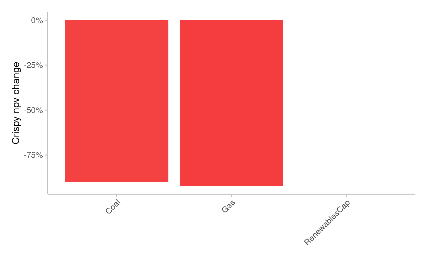

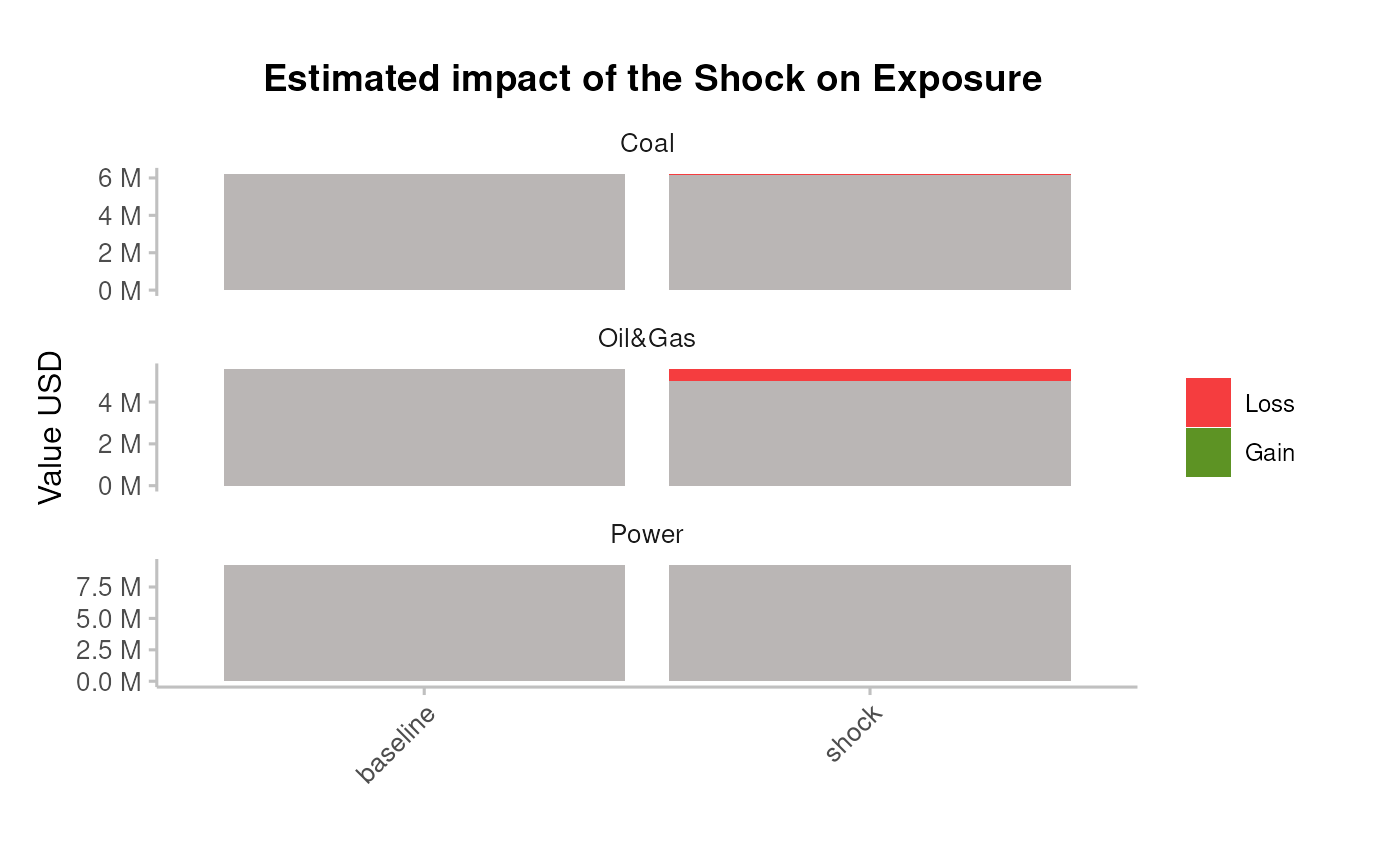
Plot the resulting portfolio’s exposure change

pipeline_crispy_exposure_change_plot(analysis_data)
#> Joining with `by = join_by(sector, technology)`
#> Warning: Removed 1 row containing missing values or values outside the scale range
#> (`geom_tile()`).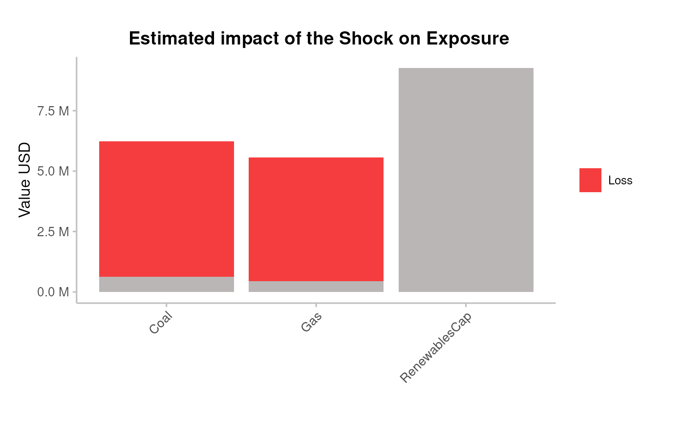

### Bonds&Loans risk

Plot the average PDs at baseline and shock

pipeline_crispy_pd_term_plot(analysis_data)
#> Joining with `by = join_by(sector, term)`
#> Warning: Removed 4 rows containing missing values or values outside the scale range
#> (`geom_bar()`).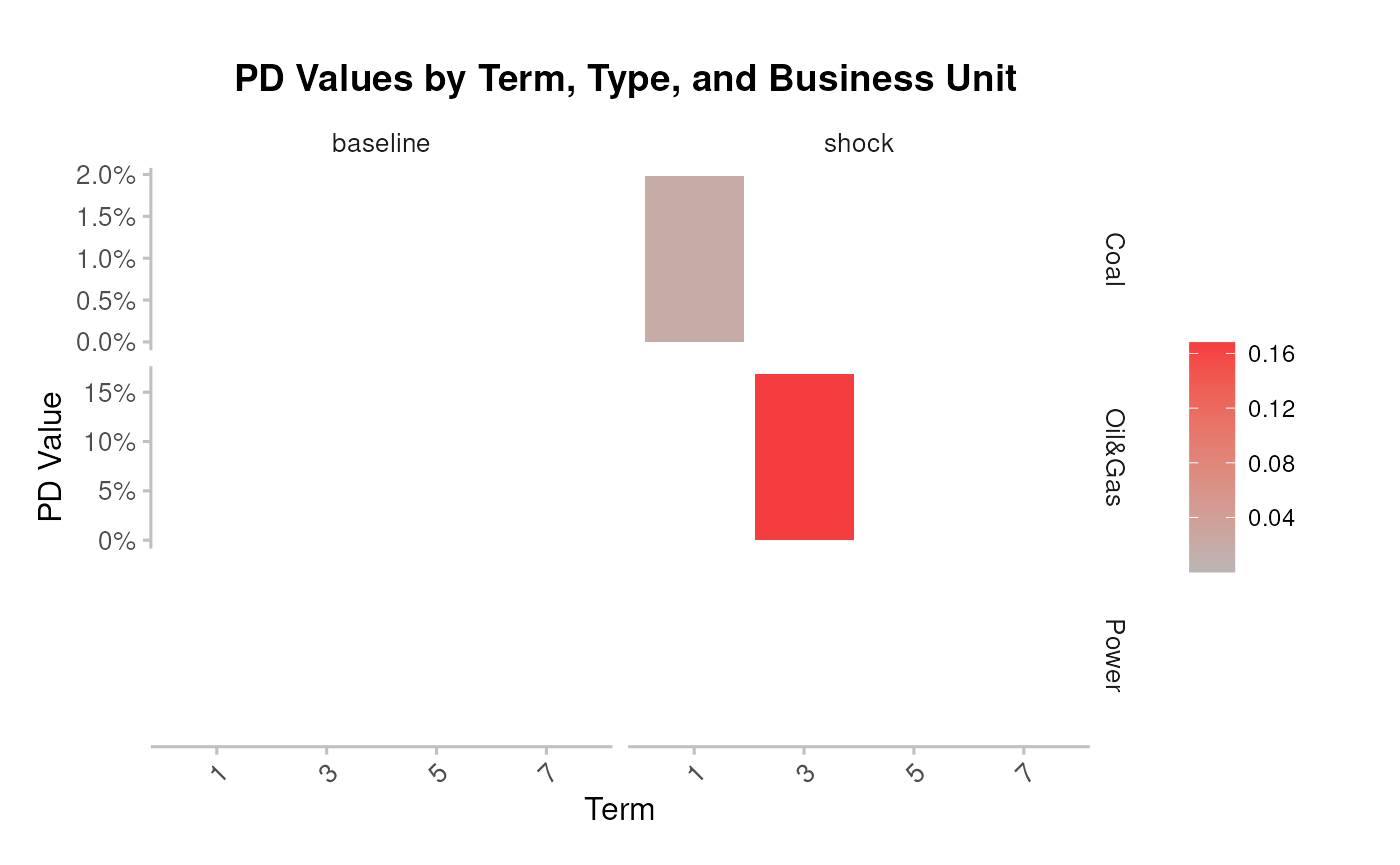

Plot the resulting portfolio’s expected loss

pipeline_crispy_expected_loss_plot(analysis_data)
#> Joining with `by = join_by(sector)`